Predictions, explained

Why explain a prediction?

A machine-learning model learns patterns from examples and uses them to make predictions about new data. In biology, those predictions may concern a protein’s function, a sample’s class or a property that is difficult to measure. Accuracy tells us how often predictions agree with a reference. It does not, by itself, tell us which information the model uses or whether that information is biologically meaningful.

Explainable artificial intelligence (XAI) studies how to make AI systems understandable to people. It includes interpretable machine learning, which develops understandable models and input representations, as well as methods that explain an already trained model. These approaches can help a researcher examine what information a prediction relies on. ^1,2

We use interpretability for understanding a model directly from its structure, without an additional explanation method. We use explainability for understanding a trained model indirectly through additional, post-hoc methods. This follows the terminology in the thesis; other authors sometimes use the terms interchangeably. ¹

The trade-off, and why it is not a law

Complex models can capture patterns that simpler models miss, but complexity does not guarantee better performance on every task. Protein sequences can also be represented through named biochemical properties such as hydrophobicity, charge and residue volume. Whether those features and an interpretable model are sufficient is an empirical question. The trade-off diagram is a conceptual guide, not a measured ranking of model classes. Rudin argues for considering interpretable models where they can meet the task’s requirements. ³

For biological prediction, an explanation can help a researcher examine whether a ranking rests on a plausible signal or an artefact in the data. It can motivate a hypothesis and a suitable comparison. Establishing a biological mechanism still requires evidence beyond predictive attribution.

Three places to put the explanation

An explanation can enter a project at three points, and they are not equivalent. Pre-modelling means building features a biologist can name before any model is trained, so that whatever the model learns is already expressed in usable terms. Ante-hoc means choosing a model whose structure can be read directly, such as a linear model or a shallow tree. Post-hoc means training a black box and then attributing its output afterwards with a separate method. ⁴

Our work starts with features that describe named physicochemical properties. That makes the input representation interpretable, but it does not automatically make every model decision transparent. Feature importance and attribution still need checks for faithfulness, stability and usefulness to the biological question.

The three names are not settled, which is itself worth knowing when reading a method paper. Carvalho's review calls them pre-model, in-model and post-model; ⁵ Ali's calls the same three data, model and post-hoc explainability; ⁴ others drop the first stage and keep only ante-hoc against post-hoc. The ground is the same and only the vocabulary moves, so a method described as ante-hoc in one paper is in-model in the next. We use the first of those throughout.

How the field divides itself

Beyond the stage, three questions separate one method from another: how far its explanation reaches, what it can be applied to, and what it hands back. The dashed boxes mark where the field has no settled vocabulary. ²

What a post-hoc method can give you

Post-hoc methods analyse a model after it has been trained. Some estimate the contribution of individual features; others find useful examples, extract rules or examine internal representations. The table groups methods by the question they address and the kind of explanation they produce. Select a method name to open its description and references.

Background: post-hoc method categories

Category	Aim	Method type	What it does	Examples
Feature attribution	Determine local and global feature importance	Perturbation-based Game-theoretic Gradient-based	Alter the input and watch the output change Analyse combinations of features Assess how sensitive a network is to its input	PFI, PDP, ICE, ALE, LIME Shapley values, SHAP LRP, integrated gradients, Grad-CAM
Example-based	Obtain representative and counterfactual examples	Prototype and criticism Counterfactual Contrastive	Find representative or atypical cases Find the smallest change that alters the output Find what must be present or absent	MMD-critic Wachter, DiCE CEM
Rule extraction	Extract logical rules	no subtypes	Derive if-then rules from the decision process	Anchors, RuleFit, LORE, TREPAN
Neural methods	Explain the mechanism and the output of a deep network	Gradient-based Concept activation Graph-based	Assess how sensitive the network is to its input Map internal states onto named concepts Identify the sub-graph or the nodes that mattered	LRP, integrated gradients, Grad-CAM TCAV GNNExplainer, XGNN
Mechanistic interpretability	Read, trace and intervene on what a network represents internally	Dictionary learning Causal intervention Circuit tracing	Split activations into sparse, nameable features Patch or ablate an activation and watch the output move Join features into the steps behind one prediction	Sparse autoencoders, InterPLM, InterProt ROME transcoders, attribution graphs
Related approaches; categories can overlap
Surrogate models	Distil what a black box knows	no subtypes	Train a white-box model on a set extended with the black box's predictions	Model distillation, InterpretML
Uncertainty estimation	Quantify the confidence of a prediction	Ensemble-based Probabilistic	Aggregate the output of several models Assess uncertainty in a Bayesian framework	Deep ensembles MC dropout, MAPIE
Causal modelling	Find and quantify cause and effect in the data	Causal discovery Causal inference	Find the underlying causal structure Estimate the causal relations	DoWhy, EconML

The categories, their aims and their subtypes follow Table 1 of the thesis, ¹ which classifies more than twenty published methods; the reviews behind the classification are cited below. ^2,4,5

The diagram below compares the same methods by scope and applicability. Local explanations concern one prediction; global explanations describe broader model behaviour. Model-agnostic methods work across different model classes, while model-specific methods depend on a particular class or its internal structure.

What this looks like in our own work

We developed Comparative Physicochemical Profiling (CPP), a feature engineering algorithm that turns protein sequences into interpretable inputs for machine learning. It compares groups of sequences and identifies features that combine a physicochemical property with a defined sequence region. We introduced CPP in our published γ-secretase study. ⁶ Our framework organises amino acid properties into named categories and reduces redundancy between scales. ^7,8

For an individual protein, SHAP attributions describe how these features contribute to its prediction. Their contributions can be mapped to sequence positions and shown alongside the structure, as in the example below. This connects the model’s prediction to biochemical properties and specific regions that a researcher can examine. ⁶

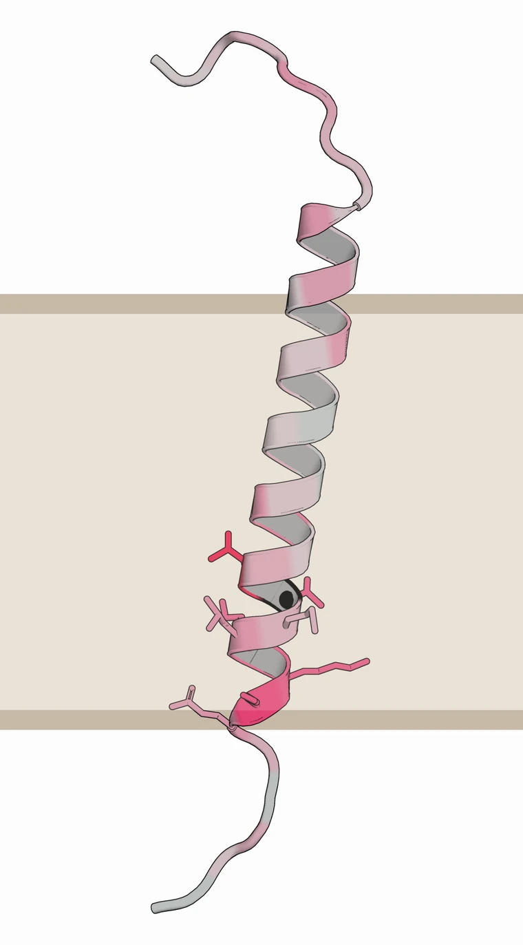
On the published γ-secretase task, optimised CPP + dPULearn reached about 90% balanced accuracy, compared with about 60% for the ProtT5 + SMOTE baseline. This task-specific result does not establish improved binder selection. Explanations make assumptions available for review and testing; they do not guarantee that the cause of a failed design is known. ⁶

What makes an explanation good

Miller's survey of the social sciences is the standard reference on this, and its four properties are a useful test for a shortlist as well as for a model. ⁹

• Contrastive. It answers "why this one and not that one", which is the question a biologist actually asks of a ranked list, and not the question most feature attributions answer.
• Selective. It gives the few reasons that carry the decision, not every feature the model touched. A ranking of two hundred features is a measurement, not an explanation.
• Social. It is addressed to someone, so the terms are the reader's and not the model's: a named property at a named position, rather than a weight on an embedding dimension.
• Causal relevance. A useful explanation can suggest a biological hypothesis to test. Predictive attribution alone does not establish a causal mechanism.

The four are a test of the shortlist as much as of the model. A method that passes all four hands a biologist something to do next; one that passes none hands them a number and the instruction to trust it.

How you would check that an explanation is any good

Miller's four properties say what a good explanation looks like. They do not say how you would measure one, and that is the harder half. Three problems block it: there are no agreed measures, there is no ground-truth explanation to compare against, and there are few benchmark datasets. Because an explanation is context-dependent and partly subjective, a universal ground truth or a single score is not a realistic goal, so what the field has converged on instead is a framework that measures several properties separately. ¹

Doshi-Velez and Kim split the measurement three ways, and the split is still the one most papers use. ¹⁰ Application-grounded evaluation puts the explanation in front of a domain expert doing the real task. Human-grounded evaluation uses non-experts on a simplified task. Functionally-grounded evaluation uses a computational proxy and no humans at all. The first two measure what you actually care about but are slow, hard to standardise and biased towards short, pleasing explanations; the third is cheap, scalable and can be optimised against, but it misses whether anyone learned anything. Only the third is a package you can install, which is worth remembering when reading a paper that reports one number.

The property that number usually claims to measure is faithfulness: whether the explanation reflects what the model actually did. Jacovi and Goldberg's point is that faithfulness is routinely confused with plausibility, which is whether a human finds the explanation convincing. ¹¹ They are independent, and an explanation can score well on the second while being wrong about the first. Around faithfulness sit three more properties that the thesis groups under fidelity: consistency, where identical inputs give identical explanations; stability, where similar inputs give similar explanations; and robustness, where a small perturbation does not change the explanation. ¹ Failing these is how a model gets the right answer for the wrong reason, the Clever Hans case. The broadest current catalogue is Nauta's Co-12, twelve properties grouped into content, presentation and user, each mapped to published quantitative measures. ¹²

Background: software for evaluating explanations

Six packages implement the functionally-grounded half. Each name opens its paper and its code.

• Quantus. The largest collection: 30 or more measures across faithfulness, robustness, localisation, complexity, randomisation and axiomatic categories, for PyTorch and TensorFlow. The default choice if you want to score an attribution. ¹³
• Captum. Infidelity and maximum sensitivity, sitting beside the attribution methods themselves. The easiest to add to a pipeline that is already PyTorch, and the thinnest in coverage.
• OpenXAI. Twenty-two measures of faithfulness, stability and fairness, with public leaderboards over fixed datasets and models. A benchmark for comparing methods rather than a library for auditing yours, and tabular data first. ¹⁴
• Xplique. Attribution, concept and example-based methods with their matching metrics in one library. TensorFlow first, with PyTorch supported. ¹⁵
• AIX360. IBM's toolkit: faithfulness and monotonicity beside eight explanation methods. The broadest in method types, the thinnest in measures. ¹⁶
• ferret. Six measures of faithfulness and plausibility, run across four explainers at once. Transformers only, tied to the Hugging Face hub. ¹⁷

Beside the libraries sit two tests worth running by hand. The model parameter randomisation test asks whether the explanation changes when the model's weights are randomised; several widely used saliency methods do not, which means they were never explaining the model in the first place. ¹⁸ RemOve-And-Retrain asks the same question from the data side, by deleting the features an explanation called important, retraining, and checking that accuracy falls. Both are in Quantus.

Prediction accuracy and explanation quality answer different questions. A model can perform well on independent data while an explanation fails to reflect how it reached those predictions. Wet-lab experiments test biological hypotheses arising from the analysis; they do not by themselves establish that an attribution is faithful to the model. ¹¹

Background: a short history of explainable AI

Earlier model classes and more recent explanation methods are shown together in the timeline below, following the historical overview in the thesis. ¹ The purple entries extend the figure with selected work on mechanistic interpretability.

For our own work the relevant part is narrow. These methods are a way to read a protein language model's embedding after the fact, and they are the strongest answer yet to the objection that embeddings cannot be interpreted at all. They are still post-hoc: the features are discovered rather than chosen, they have to be named by hand or by another model afterwards, and the naming is not guaranteed to be stable. On the published γ-secretase task our own pre-modelling features were both more accurate and already named, so we have had no reason to switch. Where we expect to use them is as a check on a model we did not build.

References

1. Our workBreimann S. Interpretable machine learning-based protein prediction. Doctoral thesis, Technical University of Munich (2025). mediatum.ub.tum.de/1763035
2. Barredo Arrieta A et al. Explainable artificial intelligence: concepts, taxonomies, opportunities and challenges toward responsible AI. Information Fusion 58, 82 (2020). 10.1016/j.inffus.2019.12.012
3. Rudin C. Stop explaining black box machine learning models for high stakes decisions and use interpretable models instead. Nature Machine Intelligence 1, 206 (2019). 10.1038/s42256-019-0048-x
4. Ali S et al. Explainable artificial intelligence: what we know and what is left to attain trustworthy artificial intelligence. Information Fusion 99, 101805 (2023). 10.1016/j.inffus.2023.101805
5. Carvalho DV, Pereira EM, Cardoso JS. Machine learning interpretability: a survey on methods and metrics. Electronics 8, 832 (2019). 10.3390/electronics8080832
6. Our workBreimann S et al. Charting γ-secretase substrates by explainable AI. Nature Communications 16, 5428 (2025). 10.1038/s41467-025-60638-z
7. Our workBreimann S, Kamp F, Steiner H, Frishman D. AAontology: an ontology of amino acid scales for interpretable machine learning. Journal of Molecular Biology 436, 168717 (2024). 10.1016/j.jmb.2024.168717
8. Our workBreimann S, Frishman D. AAclust: k-optimized clustering for selecting redundancy-reduced sets of amino acid scales. Bioinformatics Advances 4, vbae165 (2024). 10.1093/bioadv/vbae165
9. Miller T. Explanation in artificial intelligence: insights from the social sciences. Artificial Intelligence 267, 1 (2019). 10.1016/j.artint.2018.07.007
10. Doshi-Velez F, Kim B. Towards a rigorous science of interpretable machine learning. arXiv , (2017). 10.48550/arXiv.1702.08608
11. Jacovi A, Goldberg Y. Towards faithfully interpretable NLP systems: how should we define and evaluate faithfulness?. Proceedings of the 58th Annual Meeting of the Association for Computational Linguistics , 4198 (2020). 10.18653/v1/2020.acl-main.386
12. Nauta M et al. From anecdotal evidence to quantitative evaluation methods: a systematic review on evaluating explainable AI. ACM Computing Surveys 55, 1 (2023). 10.1145/3583558
13. Hedström A et al. Quantus: an explainable AI toolkit for responsible evaluation of neural network explanations and beyond. Journal of Machine Learning Research (2023). jmlr.org/papers/v24/22-0142
14. Agarwal C et al. OpenXAI: towards a transparent evaluation of model explanations. Advances in Neural Information Processing Systems 35, 15784 (2022). 10.48550/arXiv.2206.11104
15. Fel T et al. Xplique: a deep learning explainability toolbox. arXiv , (2022). 10.48550/arXiv.2206.04394
16. Arya V et al. One explanation does not fit all: a toolkit and taxonomy of AI explainability techniques. arXiv , (2019). 10.48550/arXiv.1909.03012
17. Attanasio G, Pastor E, Di Bonaventura C, Nozza D. ferret: a framework for benchmarking explainers on transformers. arXiv , (2022). 10.48550/arXiv.2208.01575
18. Adebayo J, Gilmer J, Muelly M, Goodfellow I, Hardt M, Kim B. Sanity checks for saliency maps. Advances in Neural Information Processing Systems 31, 9505 (2018). 10.48550/arXiv.1810.03292
19. Meng K, Bau D, Andonian A, Belinkov Y. Locating and editing factual associations in GPT. Advances in Neural Information Processing Systems 35, 17359 (2022). 10.48550/arXiv.2202.05262
20. Elhage N et al. Toy models of superposition. Transformer Circuits Thread , (2022). 10.48550/arXiv.2209.10652
21. Cunningham H, Ewart A, Riggs L, Huben R, Sharkey L. Sparse autoencoders find highly interpretable features in language models. arXiv , (2023). 10.48550/arXiv.2309.08600
22. Dunefsky J, Chlenski P, Nanda N. Transcoders find interpretable LLM feature circuits. arXiv , (2024). 10.48550/arXiv.2406.11944
23. Simon E, Zou J. InterPLM: discovering interpretable features in protein language models. Nature Methods 22, 2107 (2025). 10.1038/s41592-025-02836-7
24. Adams E, Bai L, Lee M, Yu Y, AlQuraishi M. From mechanistic interpretability to mechanistic biology: training, evaluating, and interpreting sparse autoencoders on protein language models. Proceedings of Machine Learning Research (2025). proceedings.mlr.press/v267/adams25a
25. Ameisen E, Lindsey J, Pearce A, Gurnee W et al. Circuit tracing: revealing computational graphs in language models. Transformer Circuits Thread (2025). transformer-circuits.pub/2025/attribution-graphs